A container of fixed width and height w,h∈R+
is filled with n∈N
(natural numbers without 0)
squares positioned in a grid‑like fashion. The squares should cover as
much of the w×h
area as possible without overflowing, which means we must maximize the
side length S∈R+
of the square. In other words, we are searching a b×a∈N2
grid which fits all our n
squares and itself fits in the container while either being as wide or
as tall as the container.
We can state the problem in a formal manner as follows:
To further clarify the last step: since s
is in the denominator, maximizing it means a
must take the smallest value greater than or equal to RHS. Since a∈N
this is precisely RHS rounded up.
Knowing a
we can now determine the side length s:
as=w⟹s=aw(3)
Since the implications in (1)
go in one direction only, we must check that s∈Sol.
The first necessary condition is:
n≤⌊sw⌋⋅⌊sh⌋(4)
since a=⌊w/s⌋
and b=⌊h/s⌋
provide the number of squares the grid should have on each
dimension, if it fits the squares and doesn’t overflow. Moreover, as=w⟹a=w/s=⌊w/s⌋,
since a∈N.
In case (i)
we can take b=⌊h/s⌋,
which means bs≤h.
Thus, s
as determined above is in Sola⊆Sol.
But in case (ii),b=⌊h/s⌋⟹n>ab⟹s∈/Sol.
A new solution s′
must be found.
Sadly, this algorithm sometimes fails to find the optimal solution.
For example, inputs:
w=10,h=2,n=8
expect S=1.25
but this algorithm gives S=1
w=7,h=2,n=20
expect S=0.7
but this algorithm gives S=0.(6)
and many others
What do these inputs have in common? When does this algorithm have
issues?
To investigate this, let’s simplify our solution statement. Observe
that:
sw∈Sola⟺sh∈Solb⟺asw=w∧bsw≤h⟺a≥rb∧sw=awwbsh=h∧ash≤w⟺rb≥a∧sh=bhhwith n≤ab for all of the above(9)sw∈Sola⟺⟺sh∈Solb⟺⟺with n≤asw=w∧bsw≤ha≥rb∧sw=awwbsh=h∧ash≤wrb≥a∧sh=bhhab for all(9)
We’ve simplified width and height to just their ratio, r=hw.
Moreover, we don’t need the side lengths themselves to compare them. Let
sw=aww,sh=bhh.
Then:
awbhs=min{a∈N:∃bw . a≥bwn∧a≥rbw}=min{b∈N:∃ah . b≥ahn∧b≥rah}={sw=awwsh=bhh if aw<rbh, otherwise(11)
The problem is reduced to just a,b
and r.
This simplification unlocks a powerful geometric representation in the
2D plane: we’re looking for points (aw,bw),(ah,bh)∈N2
such that they’re on or above the hyperbola xy=n
while accounting for their position relative to the line x=ry.x=a
is used as stand‑in for columns in the continuous space, y=b
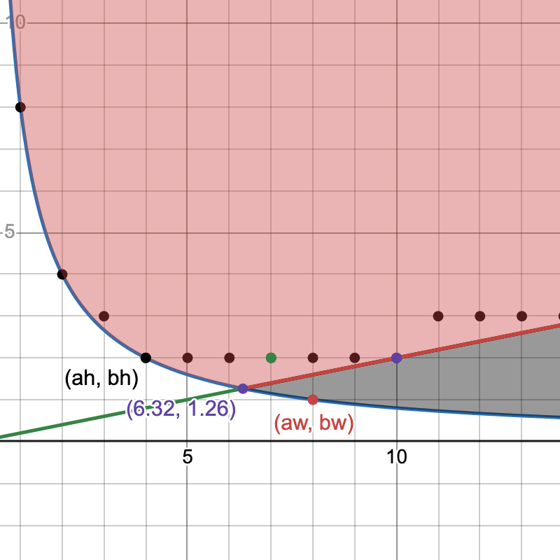
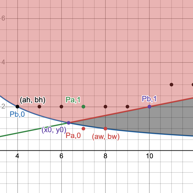
for rows. Take a look (graph A; full visualizer
here):
This is the graph for the n=8,w=10,h=2
example above, with r=10/2=5.
The black area under y=rx
contains all fit‑width solutions, the red area all the fit‑height
solutions. The union of these two contains the entire solution space,
all (a,b)
for which n≤ab,
i.e. all grid dimensions which fit all squares. Points on the green‑red
line x=ry
are grid dimensions having the ratio exactly r.
Black points are a subset of other solution candidates.
The symmetry of the problem with respect to ratio can now be directly
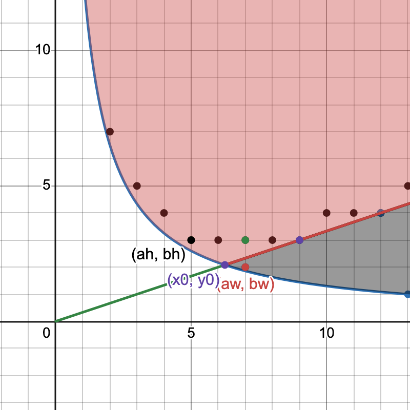
visualized. For n=13
and r=3,
respectively r=1/3,
we have:
Terminology‑wise, from here on (aw,bw),(ah,bh)
will be called a fit‑width point, respectively a fit‑height
point, if the points respect the requirements in (9);
if the points are those described in (11),
they’ll also be called minimal points (minimized coordinates
for maximal side‑length). sw
and sh
will be called fit‑width and fit‑height solutions;
unless explicitly mentioned, the (aw,bw),(ah,bh)
points implied by sw
and sh
are not necessarily minimal. Sometimes only aw
or bh
will be mentioned but keep in mind that by definition they do have a
pair bw
and ah.
Let’s now analyze the solution space.
First, notice the purple point at the intersection of the hyperbola
and the line – that is, the (x0,y0)
where y0n=ry0
– is special. This would be the “ideal” point, if rows and columns could
be fractional somehow: only these dimensions exactly fit all squares and
have the exact desired ratio. Notice that:
The number of columns a
chosen in (2)
is precisely ⌈x0⌉.
This is the visual confirmation of that result: all the fit‑width points
will find themselves to the left of that point, all the fit‑height
points to its right. In other words:
∀aw,bh . aw≥x0∧bh≥y0(13)
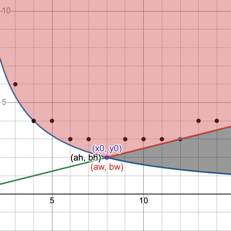
If parameters are “nice” such that x0,y0∈N
the minimal fit‑width and fit‑height points coincide (graph B):
Second, when is a point valid, i.e. satisfies solution
requirements in (9)?
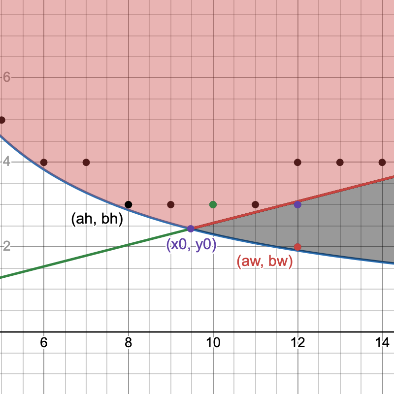
Also, can multiple points give the same solution? Consider the following
(n=23,r=3.9,
graph C):
The 4 points next to (ah,bh)
have the same ordinate and the point above (aw,bw)
the same abscissa, therefore their corresponding side lengths are still
sh,
respectively sw.
This follows directly from the solution requirements in (9):
Fit width:awbw≥n∧aw≥rbw⟺⟺Fit height:ahbh≥n∧bh≥rah⟺awn≤bw≤raw⌈awn⌉≤bw≤⌊raw⌋⌈bhn⌉≤ah≤⌊rbh⌋(14)Fit width:awbw≥n∧aw≥rbw⟺awn≤bw≤raw⟺⌈awn⌉≤bw≤⌊raw⌋Fit height:ahbh≥n∧bh≥rah⟺⌈bhn⌉≤ah≤⌊rbh⌋(14)
We can add the ceiling and floor as a consequence of them being
residuated mappings. Notice how the intervals describe the space between
the hyperbola and the line for ah
and bw.
Doesn’t matter which value from these intervals ah
and bw
have, the solutions of (aw,bw),(ah,bh)
are the same. The ceilings and floors are visible in the graph too: the
points are a bit above/under the function graphs too. We can compress
the inequality to get the validity condition:
The number of points with equal solutions is easily derived by
subtracting the interval endpoints.
Third, which points give the optimal solution s?
How do they compare? Recall (10):
sw>sh⟺aw<rbh
From (9)
we know that for any (ah,bh)
fit‑height point, ah≤rbh,
meaning rbh
is an upper bound on a fit‑height solution’s number of columns.
Therefore:
A fit‑width point with less columns than some fit‑height
point gives the better solution between the two.
If rbh∈/N
then both aw≤⌊rbh⌋
and ah≤⌊rbh⌋,
meaning they can have at most as many columns. This is unsurprising: the
fit‑width solution stretches the columns fully, while the fit‑height
doesn’t.
What about the number of rows? Since aw≥rbw
we get that:
A fit‑width point must have less rows than a fit‑height point to
correspond to a better solution.
It makes sense intuitively: a fit‑height solution stretches the rows
fully, a fit‑width doesn’t; if a fit‑width solution has as many rows or
more, it must be worse.
We can observe these properties on the graphs above:
in graph A the fit‑width solution has less
columns: it is the better one
in graph C the fit‑width solution has more
columns: it is worse
Graph C shows that having less rows doesn’t matter, since one can
simply add more rows. Mathematically, for (aw,bw)
fit‑width, (ah,bh)
fit‑height points, if sw≤sh:
Fourth and finally, when r≥1
if the minimal fit‑width solution is strictly better than any fit‑height
solution, then it corresponds uniquely to a single point (prove it
yourself! or see appendix for proof). Symmetrically for r<1
the same applies for the fit‑height solution.
We can now analyze when the algorithm we’ve developed fails.
Translating its solution to points:
Recall that if a fit‑width point has a solution greater than that of
a fit‑height point it will have less rows. Above we can see that all of
Pa,1,Pb,0,Pb,1
have a number of rows greater than y0:
for Pb
it is by construction, and for Pa,1:
⌈raw⌉=⌈r⌈rn⌉⌉≥r⌈rn⌉≥rn=y0
Moreover, for r≥1
there exists a fit‑height solution with bh=⌈y0⌉
with very high probability and fit‑width solutions with aw=⌈x0⌉
are highly unlikely – in fact, almost never likely for r≥2
(see appendix for proof). Therefore, the optimal solution mainly
corresponds to a unique fit‑width point (aw,bw)
with aw>⌈x0⌉
and bw<⌈y0⌉
yet the algorithm is optimized to find a fit‑height point (ah,bh)
with ah≤⌈x0⌉
and bh≥⌈y0⌉.
By the conclusions in the appendix, the outcome is predominantly
ratio‑dependent; for the vast majority of ratios the algorithm does not
find the optimal solution (e.g. r∈[1.5,2)
paired with most n).
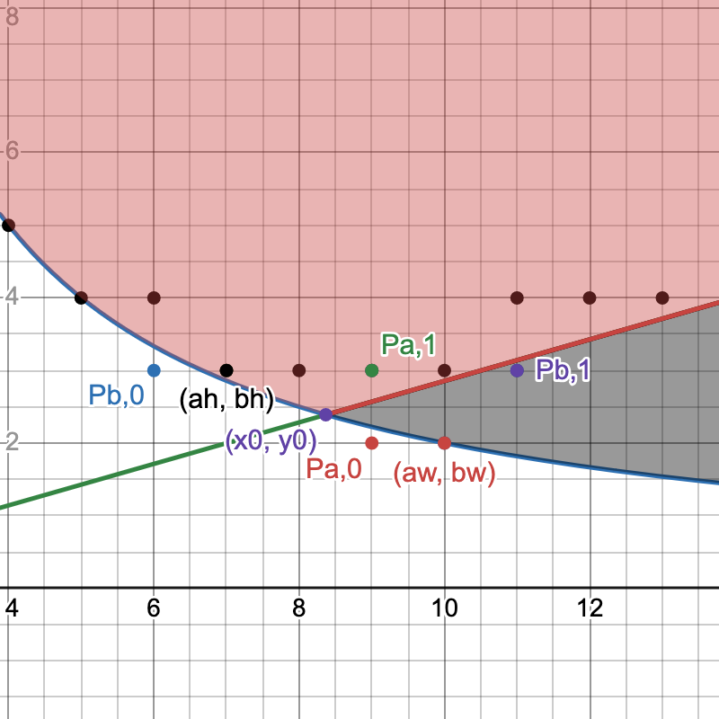
Let’s visualize this on the graphs of the two counterexamples given
above (r=5,n=8
and r=3.5,n=20):
The initial fit‑width point candidate Pa,0
is invalid in both cases (under the hyperbola), so the algorithm falls
back to Pa,1,
a fit‑height point. In the first example, Pb,0
is already valid, so the fallback Pb,1
is not used; in the second, the fallback is used instead but even though
it’s a fit‑width point its solution is equivalent to the fit‑height
solution, as they have the same number of rows.
Let’s now build a new algorithm. This algorithm should find the
minimal fit‑width and fit height points and pick the solution with the
greater side length. Using (15)
, the solution we’re looking for is:
Let’s walk through how we translate this to code. First, we are
looking for minimum aw
and bh;
from (13)
we know that aw≥⌈rn⌉
and b≥⌈rn⌉.
We’ll initialize variables a and
b to those values. Then we need to ensure the
validity condition; for that, we just increment
a and b in a loop
until the condition holds. The loops execute while aw
and bh
are invalid points:
⌈an⌉>⌊ra⌋⟺a<r⌈an⌉⌈bn⌉>⌊rb⌋⟺rb<⌈bn⌉(17)
The implementation follows directly:
const r = w / h;
let a = Math.ceil(Math.sqrt(r * n));
for (; a < r * Math.ceil(n / a); a++);
let b = Math.ceil(Math.sqrt(n / r));
for (; r * b < Math.ceil(n / b); b++);
returnMath.max(w / a, h / b);
The algorithm always terminates: as a
grows, ⌈an⌉
decreases and ⌈ra⌉
increases, shrinking the interval until the ordering of its endpoints is
swapped; likewise for b.
The values at the end of each loop are minimal – we check every value
one by one in ascending order.
Intuitively, if the loop condition holds there is no valid (aw,bw)
or (ah,bh)
fit‑width, respectively fit‑height point with the iteration’s current
aw
or bh
value. If we take bw=⌈an⌉
and ah=⌈bn⌉
(the minimum values for a valid solution) we can imagine this algorithm
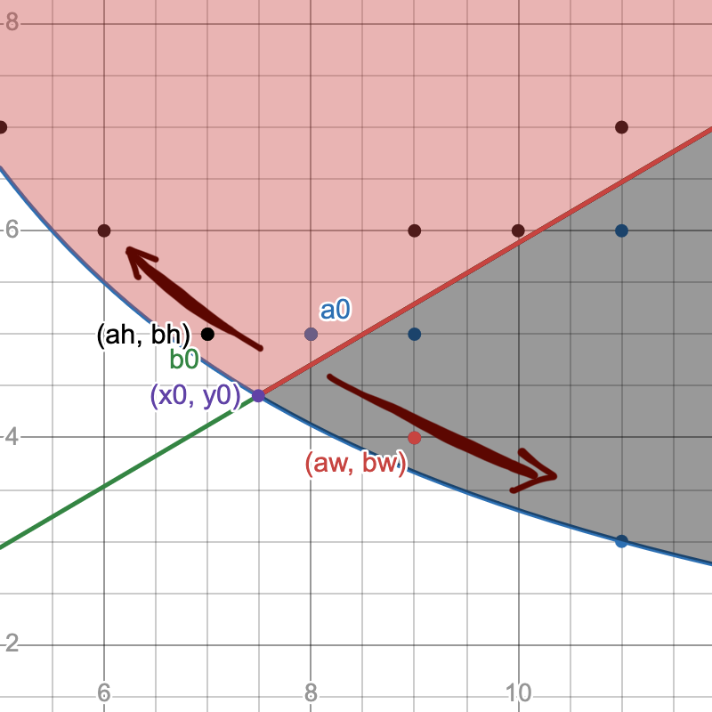
as “walking away” from (x0,y0)
alongside the hyperbola until we (inevitably) find ourselves in the
fit‑width/fit‑height solution spaces:
a0
and b0
are the starting points, right next to (x0,y0).
The algorithm “walks down” to (aw,bw)
and “up” to (ah,bh).
In fact, in this example, b0
is initialized directly to (ah,bh);a0
must be incremented once.
We have convinced ourselves of correctness. To analyze its runtime
complexity, let’s denote a0=⌈rn⌉
the starting value of a.
Since the loop condition is a<r⌈an⌉,a
will be incremented at most ⌈r⌈an⌉−a0⌉
times. Since a
increases ⌈an⌉≤⌈a0n⌉.
We can now count iterations:
This means at most ⌊r⌋+1
iterations and a runtime of O(r),
dependent only on the aspect ratio of the grid. To show that the bound
is tight, consider this following example:
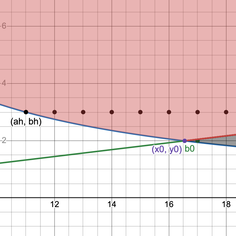
Here n=33,r=8.3.
A very rare case when the fit‑height starting point b0
is in the fit‑width solution space. Consider the iteration count of the
fit‑height loop of the algorithm – by the same reasoning it is ⌊r1⌋+1.
It’s visible that in this example the loop will do exactly 1 iteration
to reach (ah,bh).
Since the algorithm is symmetric this proves tightness for the first
loop by using the same n
and r′=r1.
With a correct algorithm and good understanding of why it works, we
conclude here.
Appendix
Uniqueness of
fit‑width solution when r≥1
Let (a,b)
be a minimal fit‑width point. We prove there is no b′
such that (a,b′)
is a fit‑width point when r≥1
and (a,b)
corresponds to the best solution, meaning that sw>sh
for all (ah,bh)
fit‑height points.
Assume towards a contradiction there exists b′=b
such that (a,b′)
is a fit‑width point. Without loss of generality, we can further assume
b<b′.
From (14)
and the minimality of a
we can write a
in terms of b′:
n≤ab′∧a≥rb′⟹a≥⌈b′n⌉∧a≥⌈rb′⌉⟹a=max{⌈b′n⌉,⌈rb′⌉}
Suppose that a=⌈b′n⌉.
Since we have n≤ab
from (14),b<b′
and r≥1:
a−1<b′n⟹b′(a−1)<ab⟹(b′−b)a<b′⟹a<rb′
But a≥rb′
so we’ve reached a contradiction. Therefore, together with the first
result:
a=⌈b′n⌉⟹⌈b′n⌉<⌈rb′⌉=a⟹⌈b′n⌉≤⌊rb′⌋
By (14)
this means for integer ⌈b′n⌉≤a′≤⌊rb′⌋
the point (a′,b′)
is fit‑height (real example in graph C). But
then, since for this one fit‑height point sh=b′h:
a≥rb′⟹sw≤sh
In conclusion, b′=b
contradicts sw>sh,
thus b′
can’t exist and (a,b)
is unique.
Position of
solution points relative to (x0,y0)
We’ll approach this subject by handling fit‑height points where r≥1.
Due to the symmetry of the problem relative to ratio, we can make more
general conclusions afterwards.
b=⌈y0⌉=⌈rn⌉
is a valid fit‑height point by (15)
if and only if:
If b
is greater than that the fit‑height point (a,b)
is valid. The condition excludes cases when ∃k∈N . k∈[bn,rb]
(e.g. when y0∈N
then the point valid for every n)
but it is easy to quantify. We can use it to answer: for fixed
r≥1
what’s the probability for b
to be a valid fit‑height solution?
To do this, observe that by the properties of ceiling, rn≤b<rn+1.
We can bound the expression above likewise, using r≥1:
rn<2r1+4r21+rn<21+(21+rn)2=rn+1
It follows that:
rn<2r1+4r21+rn≤b=⌈rn⌉<rn+1
If we subtract rn,
the difference will be always between 0
and 1:
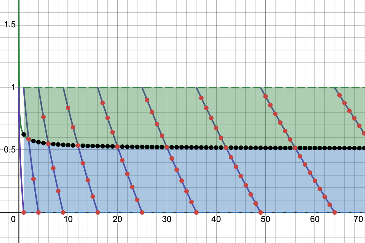
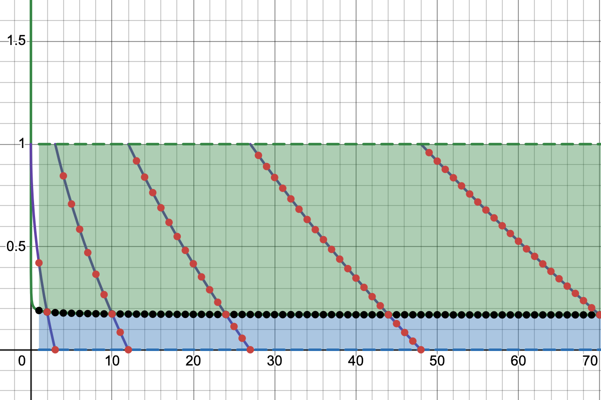
First graph depicts r=1,
the second r=3.
The red points represent Cr(n),
the black points Br(n).
Whenever a red point is in the green area Cr(n)≥Br(n),
meaning ⌈rn⌉
is a valid fit‑height point for n.
Since this criterion doesn’t cover all possibilities, the ratio
between the number of valid points in the green area and the total
number of points provides a lower bound for the probability that b
is a valid point:
This tells us that a percentage of 1−t
points out of n
are in [t,1].
One can roughly notice this on the graph: the points (n,Cr(n))
are distributed
uniformly between the green and blue areas, proportionally with
their sizes.
The limit’s numerator is equivalent to {k∈[n]:Cr(k)≥t}.
For t=Br(k)
this would’ve been precisely Sn,
with the limit then giving us d(S)
directly, but t
must be constant. To find an appropriate value, let’s bound Br(n):
The approximation 1+x≤1+2x
was used. Observe that the second term vanishes as n→∞.
There may be an initial finite interval on which it excludes numbers,
but for the remaining infinite tail it changes nothing. Since the
density of a finite subset of integers is 0,
we can ignore that segment when computing d(S).
The effect is also visible on the graph early on.
This means we can simply take t=limn→∞Br(n)=2r1.
Our final result is:
As a final note, attempting to exclude points where Cr(n)=0,i.e. rn∈N,
would’ve not influenced the result. rn∈A,
where A={p2p∈N}
the set of all squares, and since ∣A∩[n]∣≤O(n),d(A)=0.
Our set of points is a subset of that, so it must also be
density‑zero.
The first conclusion is that fit‑height solutions will for the most
part have bh=⌈rn⌉.
We can derive even more interesting information by looking at the graph
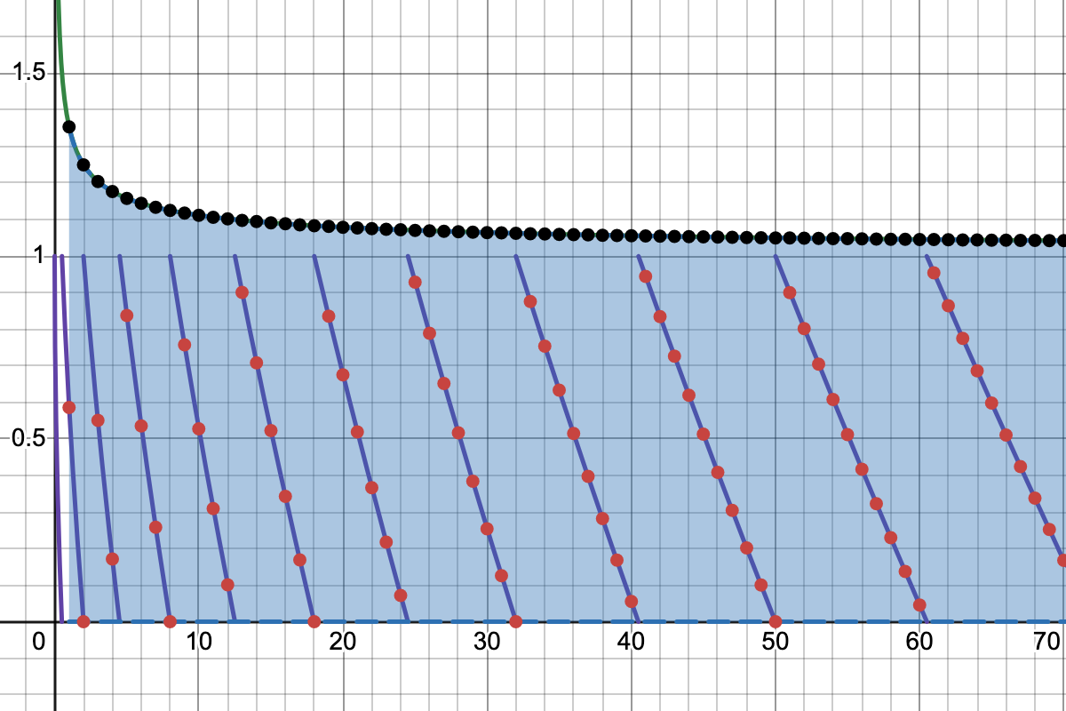
for r<1:
Note that r<1
means we’ve essentially flipped dimensions: the fit‑height points
correspond to the fit‑width points of ratio r1.
For r=21
as depicted above, P21≥0.
How do we interpret this?
For r≥2,
no a = ⌈rn⌉
satisfies the sufficient condition above to fulfill the fit‑width
solution requirements.
Any valid aw
will be greater than ⌈x0⌉
with very high certainty, especially when considering the growth rate of
2r1
as r→0.
This also provides an intuitive explanation for the second algorithm’s
runtime: as r
grows the fit‑width solutions are farther and farther away from (x0,y0),
so the first loop will have to iterate more; at the same time, the
probability that the initial fit‑height solution candidate is valid
rapidly increases, which prevents the second loop from iterating.
The final conclusion is: for r≥1
it is very likely that bh=⌈rn⌉
is a valid fit‑height point and almost never likely that aw=⌈rn⌉
is a valid fit‑width point. Then mostly bw<bh,
since with more columns the grid requires less rows to fit all squares.
Therefore by (17)
for r≥1the fit‑width solution is in the majority of cases better than any
fit‑height solution. Likewise for r<1
but with fit‑width and fit‑height swapped.
Using binary search
in the second algorithm
According to (18)
the algorithm always finds a solution after ⌊r⌋+1
iterations, thus a0≤aw<a0+r+1,
where a0=⌈rn⌉
is the starting value for aw.
We can binary search over that interval using the same loop condition
from (17).
If the midpoint is not a valid aw,
we search in the upper half, since we’re not yet in the solution space,
otherwise we search in the lower half, since we want the minimal
solution. Here is the algorithm for aw:
const r = w / h;

let left = Math.ceil(Math.sqrt(r * n));
let right = Math.ceil(left + r + 1);

while (left < right) {
  const mid = Math.floor(left + (right - left) / 2);
  if (mid < r * Math.ceil(n / mid)) {
    left = mid + 1;
  } else {
    right = mid;
  }
}

return w / left;
Upper bound ceiled so interval is open.
left stores aw.
This reduces the asymptotic runtime to O(logr).
Useful for very large ratios but very large ratios seem utterly
useless.
⌊⋅⌋
and ⌈⋅⌉
are residuated mappings
This means that, for ∀x∈R,n∈N:
n≤x⟺n≤⌊x⌋
x≤n⟺⌈x⌉≤n
n<x⟺n<⌈x⌉
x<n⟺⌊x⌋<n
To prove the first, if x∈N
then clearly n≤⌊x⌋=x,
else if x∈R∖N:
The others are proven in a similar fashion. Read more about this on
Wikipedia’s
“Equivalences” for floor and ceiling. These are standard properties
but I insisted on writing them here as a “note to self” since I’ve
confused myself and applied them wrong way too many times. I probably
know that Wikipedia page now by heart.